A Reader's Guide to Machine Learning in Hematology

“Where is the wisdom we have lost in knowledge? Where is the knowledge we have lost in information?” – T.S. Eliot, The Rock

A quick PubMed search will reveal that the introduction of machine learning (ML) into the medical literature has been following an exponential curve. However, many clinicians remain unsure of what machine learning is, how it works, and what advantages and limitations it holds. In this Morning Report we hope to introduce key concepts and terms encountered in articles using machine learning techniques as well as lay out what we believe are some of the key pitfalls to be aware of when reading and considering studies using ML approaches.

What is machine learning?

Machine learning is a subfield of artificial intelligence (AI) in which computer algorithms identify arbitrarily complex patterns in data. The computer can “learn" patterns directly from large sets of data without being explicitly programmed. This contrasts with traditional statistical approaches in which hypotheses and rules (the model) are defined a priori. At its best, machine learning holds the promise of identifying meaningful patterns in datasets whose size renders them impossible to interpret by mere human capacity. Such models are commonplace in our society; for instance, sophisticated online retailers use ML to analyze every action taken on their website — down to how long a user lingers looking at a particular item — to better predict what the user would be interested in buying. Self-driving cars are “taught” to recognize other vehicles, pedestrians, and stop-lights through ML algorithms which can rapidly perceive and respond to visual data. In medicine, ML tools are already implemented in image-recognition settings such as recognizing large vessel occlusion and intracranial hemorrhage on computed tomography of the head (Avicenna.AI, Brainomix, RapidAI). In oncology, the development of image-recognition applications that use ML to identify malignant skin lesions from photographs, breast lesions on mammography, and to estimate Gleason scores from digitized slides of prostate tissue, all with accuracy on par with that of experienced clinicians.1

What does ML do differently from traditional statistics? Take the following example: A two-dimensional grid with points in red or blue (Figure 1A). A straightforward linear model, defined by slope and intercept (like the sort learned in grade-school algebra class) does an acceptable job of segregating the two colors (Figure 1B). More red dots and fewer blue dots are on the upper left, which this model captures. Twelve of 17 dots are on the correct side, showing 71 percent accuracy. This is a gross oversimplification but this model is conceptually akin to a traditional statistical model and can be defined by a set of specifiable, interpretable rules. Now consider the third version (Figure 1C). Here, the line separating the red-dot compartment from the blue-dot compartment is 88 percent accurate, a substantial improvement. A mathematical function describing the separation line in this version would be more challenging to define – perhaps not impossible, but imagine extending the example from two dimensions to hundreds or thousands, and it is easy to see why this problem exceeds the capacity of a human-predefined set of rules. Fed enough raw data, these sorts of patterns in information are where ML excels.

Figure. Machine Learning in Two Dimensions

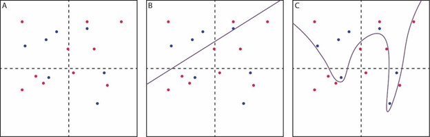
(A) red and blue dots are scattered across a two-dimensional grid. (B) a simple linear model (slope and intercept) is used to segregate the red and blue dots, but with only modest accuracy. (C) a complex model is used to segregate the red and blue dots, achieving improved accuracy with a non-linear boundary between the groups that would be difficult to approximate with a single mathematical function (and much more difficult in a high-dimensional version of this problem).

Note the single blue dot which “teaches” the model to include a very narrow region on the right side of the plot. This may suggest overfitting, which is when a model comprises rules so specific to the particular cases in the original data that these rules are not easily generalized to other data sets. This is an important pitfall in ML which we will discuss again below.

Types of ML:

ML is generally divided into two major categories:

• Supervised learning: In supervised learning, an ML algorithm is “trained" on labeled data. For instance, in order to predict complete remission following induction for acute myeloid leukemia, the model might draw on a set of baseline variables for thousands of patients who underwent treatment, with each patient record labeled as having achieved remission or having failed to achieve remission. Similar techniques can be used with image recognition, where the algorithm is trained on thousands of photographs of peripheral blood smears (“training set”), which are labeled with the associated diagnosis in order to develop a model that can predict diagnoses from new (“test set”) smears.
• Unsupervised learning: In unsupervised learning, the algorithm is fed data without any labels and is designed to independently identify patterns within the data. These methods are particularly common in -omics settings, such as in single-cell RNA sequencing analyses where unsupervised learning can be used to identify clusters of similar cells. These clusters may then be labeled and further explored by the investigator by including additional information not included in the clustering model.

Most published models designed for clinical practice are examples of supervised learning, used to predict diagnosis, risk of treatment failure, or durability of treatment response.

Supervised learning algorithms:

There are numerous approaches to supervised learning, each with its own set of variations on a theme. We discuss three of the most commonly-encountered approaches here. The first two, random forests and gradient boosting, are generally rooted in the idea of “decision trees.” Decision trees function by progressively splitting a dataset by different binary predictors into narrower groups, like a tree with its trunk, great branches, smaller branches, and twigs. The “leaves” at the end are the final subgroups for which individual predictions can be made. For instance, we might have a tree in which the cohort is split first by age — greater than versus less than 50 years. The next branching point, among the patients younger than 50 years, are split by a baseline hemoglobin of less than versus greater than 10 g/dL, and so on. A final prediction (say, a risk group, or likelihood of 1-year overall survival) is reached by following these branches to the furthest point. Random forests and gradient boosting both take advantage of the computer’s ability to generate a multitude of such trees to fit a set of data, combining their predictions in different ways:

• Random forests: Random forests are considered an "ensemble” or collection of many individual decision trees. Each is created from a unique, random subsample of the full data. In developing the individual trees, the particular variables from which any branching point can be selected come from a randomly-selected subset of all possible variables in the model. This strategy limits the correlation between different trees in the forest, forcing greater variation into the model. Once numerous individual trees are developed, predictions can be made for a new case, often by taking the “majority vote” (modal prediction) or averaging across the individual trees. Random forests are felt to minimize the problem of overfitting. Random survival forests are a special case of random forests which accommodate right-censored data (i.e., survival outcomes).
• Gradient boosting: Gradient boosting also typically starts with a decision tree. In this case, however, a single tree is generated, and its predictive accuracy is determined. An adjustment is made to the tree to decrease its predictive error, generating a new tree. This process is repeated iteratively, each tree improving on the prediction of the former. The final prediction is an average of all trees, weighted by each tree’s predictive accuracy. In contrast to random forests, gradient boosting has a higher risk of overfitting.
• Deep learning: Also known as artificial neural networks, this domain of ML potentially has the greatest power but often requires enormous quantities of data to generate useful predictions. Deep learning begins with an individual “neuron.” Here, we have familiar algebra; though it’s often described using matrices instead, the basic idea is that a series of variables or inputs labeled xi are multiplied by their respective coefficients, or weights, labeled wi. The sum of these, plus an intercept, or bias term, then undergoes a non-linear transformation (activation function). This transformation allows the model to fit the sorts of complex shapes we described earlier. The “deep” part of deep learning is the use of multiple layers of these neurons; the outputs of several individual neurons become inputs into a second layer of neurons, and so on. These layers upon layers are what make deep learning extraordinarily powerful (given enough data) but are also what make their interpretation challenging. Weights in the hidden layers — that is, the weights assigned to the outputs of neurons earlier in the model — have no interpretable meaning. For this reason, ML models, especially deep learning models, are often thought of as “black boxes,” their inner workings obscure.

Pitfalls:

Considering the black box of deep learning, we are reminded of Arthur C. Clarke’s famous statement, “Any sufficiently advanced technology is indistinguishable from magic.” However, machine learning algorithms are not magic. They are potentially powerful statistical tools that, when used appropriately, can yield deep insight into data exceeding our ability to comprehend. With that in mind, there are several key pitfalls that these models can often fall into, and which readers of articles using these technologies should bear in mind when considering their validity and clinical usefulness.

• Lack of interpretability: We have already introduced the concept of the black box. Contemporary ML literature has devoted significant energy to illuminating the box. In random forest models, a technique such as variable importance can provide useful insight. Data are serially permuted and fed back through the algorithm; then the impact of these permutations on predictions is used to determine which variables the model weighs most heavily in its prediction. In some cases, a second separate ML model is created for the task of learning the relationships between model inputs and predictions.
• Overfitting: As mentioned above, the danger of learning the training data too well is that a model can make excellent, precise predictions about those data but consequently make very poor predictions on external data.
• Data quality: As in any statistical setting, the classic phrase “garbage in, garbage out” applies. ML models may be even more sensitive to subtle problems of data quality, as the models may find inadvertent patterns in noise or artifact. For instance, if a set of “normal” radiographs are drawn from an older dataset than those images showing pathology, the model may learn to recognize technical qualities of newer imaging rather than radiologic features as prognostic of illness.²
• Data quantity: ML algorithms are notoriously data-hungry. Increasing numbers of cases reduces the likelihood of overfitting and increases model accuracy. There is no “golden number” at which every model saturates with enough patients or cases to generate stable, useful predictions; however, simulations suggest that the optimal number for random forest and boosting applications can be in the several thousands,3 with deep learning often requiring orders of magnitude more.⁴
• Class imbalance: This is a more subtle issue. Consider the possibility of a binary classification task – predict whether a patient belongs in category A or category B. If category B is extremely rare in the data, then an algorithm designed to maximize correct categorization will find a clever solution; always (or almost always) predict the majority category. Accuracy will be high, but the predictions will be essentially meaningless. There are several techniques which have been developed to address these situations.⁵
• Uncertainty and confidence: We are used to statistics being presented with a confidence interval, from which we can draw some inference about how certain we should be of the result. Clinical ML articles often propose models that do not provide indication of the degree of uncertainty associated with a particular result. This is an evolving field of study; one approach consists of providing the range of predictions across a large number of component sub-models. The CLL-TIM, which combines an ensemble of different ML approaches to identify risk of infection in patients with chronic lymphocytic leukemia, is an excellent example of this approach.⁶

In the realm of risk and outcome prediction using AI, an effort is currently underway to standardize best practices. The Transparent Reporting of a multivariable prediction model for Individual Prognosis Or Diagnosis (TRIPOD) statement⁷ serves as a model for the anticipated TRIPOD-AI guidelines.⁸ These statements provide a principled, rigorous approach to designing and evaluating research in individualized risk prediction.

The availability of massive data sources — electronic medical records, registries, imaging databases, -‘omics biobanks — is growing at an exponential pace. ML approaches have an important place in interrogating and drawing clinically useful knowledge from this proliferation of information. The fundamentals of biostatistics have long been thought integral to medical education, to enable understanding and criticism of the medical literature. The coming years promise to make the same true of ML as well. To address T. S. Eliot’s concern, well-constructed ML models may help rescue knowledge from information; thoughtful clinicians and scientists will still need to draw wisdom from that knowledge.

1. Elemento O, Leslie C, Lundin J, et al. Artificial intelligence in cancer research, diagnosis and therapy. Nat Rev Cancer. 2021; DOI: 10.1038/s41568-021-0039901.
2. Cabitza F, Rasoini R, Gensini GF. Unintended consequences of machine learning in medicine. JAMA. 2017;318:517-518.
3. Shouval R, Labopin M, Unger R, et al. Prediction of hematopoietic stem cell transplantation related mortality- lessons learned from the In-Silico Approach: A European Society for Blood and Marrow Transplantation Acute Leukemia Working Party Data Mining study. PLoS One. 2016;11:e0150637.
4. Wang F, Casalino LP, Khullar D. Deep learning in medicine–promise, progress, and challenges. JAMA Intern Med. 2019;179:293-294.
5. Rahman MM, Davis DN. Addressing the class imbalance problem in medical datasets. Intl Journal of Machine Learning and Comp. 2013;3:224-228.
6. Agius R, Brieghel C, Andersen MA, et al. Machine learning can identify newly diagnosed patients with CLL at high risk of infection. Nat Commun. 2020;11:363.
7. Collins GS, Reitsma JB, Altman DG, et al. Transparent reporting of a multivariable prediction model for Individual Prognosis or Diagnosis (TRIPOD): the TRIPOD statement. Ann Intern Med. 2015;162:55-63.
8. Collins GS, Dhiman P, Andaur Navarro CL, et al. Protocol for development of a reporting guideline (TRIPOD-AI) and risk of bias tool (PROBAST-AI) for diagnostic and prognostic prediction model studies based on artificial intelligence. BMJ Open. 2021;11:e048008.